Basic concepts
The preferences file stores labdata related configurations and is located in $HOME/labdata/user_preferences.json.
Before anything else you need to **get credentials** from your admin and write them to your **preference file**.
labdata will generate a preference file if you attempt to run a command in the command line; e.g. labdata --help.
- You need to at least set the
databasesection; these are the credentials to the database. - If you want to access data files you need to set the
local_pathsandstoragesections.local_pathsare a list of paths with the locations where labdata searches for data; it can be on the network or local or both.storageis where you store the credentials to storage . - If you need to upload data, you need to set
upload_path,upload_hostandupload_storage. This needs to be done only if the computer is putting raw data to storage - which must go through the local server, analysis data are pushed directly.
Database and storage configuration
labdata requires a mysql database, to store data and metadata related to experimental sessions. The database can also be used to store processed or analysed data and can be extended by any user - throught plugins.
To specify a database use the preference file database section:
"database": {
        "database.host": "<ADDRESS_OF_THE_MYSQL_SERVER>",
        "database.name": "<NAME_OF_THE_DATABASE_SCHEMA>",
        "database.user": "<USER_NAME>",
        "database.project": "<PROJECT_NAME>"
    },
labdata will search for files in a local paths before attempting download from a remote server. The storages can be configured on the preference file.
"local_paths": [
         "<LOCAL PATH WHERE DATA MIGHT BE FOUND>",
         "<NETWORK LOCATION TO AVOID CLOUD DOWNLOAD>"
    ],
Configuration of data stores. Data stores can be on AWS or on local file servers.
You can configure multiple stores for different purposes, for example below is configured a data storage to keep raw data files and a analysis store that is used to keep analysis by-products. Stores are configured on the preference file to allow migrations if needed.
To configure AWS storage, add the following to the preference file:
"storage": {
         "data": {
             "access_key": "<ACCESS KEY>",
             "bucket": "<BUCKET NAME>",
             "endpoint": "s3.amazonaws.com:9000",
             "protocol": "s3",
             "secret_key": "<SECRET KEY>"
         },
         "analysis": {
             "access_key": "<ACCESS KEY>",
             "bucket": "<BUCKET NAME>",
             "endpoint": "s3.amazonaws.com:9000",
             "protocol": "s3",
             "secret_key": "<SECRET KEY>"         }
     },
"allow_s3_download" : true,
The flag allow_s3_download will prevent downloading from s3 when data are not found in local_paths.
Projects
labdata Allows organizing data by projects. This is meant to be used by a research laboratory in which case experimenters might share the raw data files but keep metadata and other analysis separate. Project-based organization enables granular user permissions and isolates derived data and metadata, making it easier to share specific datasets with collaborators without exposing the entire database. This approach streamlines data export for publication and ensures that data from other projects are independent.
The File and UploadJob tables are stored on a global schema and shared across projects. This makes that data are not duplicated and can span multiple projects.
The environment variable LABDATA_DATABASE_PROJECT allows specifying the project outside of the preference file.
Local lab server
The role of the lab server is to receive data from experimental computers and apply pre-defined compression rules to data before uploading to the cloud (or stored for archival).
It can also deploy data preprocessing and other analysis locally.
A local server often is a dedicated computer running Linux and has a scheduler installed (like slurm).
labdata can run analysis on apptainer containers for reproducibility and configuration ease. Definitionfiles for default containers are in the containers folder. The command labdata build-container <CONTAINER FILE> --upload builds the container files and uploads to the analysis bucket on AWS.
Command line interface
labdata ships a command-line tool called labdata. Every sub-command accepts -h for inline help:
labdata --help
labdata <command> --help
Commands are organised into four groups based on who runs them and when.
Browsing data
These commands read from the database and are safe to run anywhere.
| Command | Description |
|---|---|
labdata subjects |
List all subjects |
labdata subjects -u <user> |
Filter by lab member |
labdata subjects -f <name> |
Filter by name substring |
labdata subjects -s M |
Filter by sex (M, F, U) |
labdata subjects --include-size |
Show raw data size per subject |
labdata sessions -a <subject> |
List sessions for a subject |
labdata sessions -a <subject> --include-size |
Include file size per dataset |
Moving data (experimental computers)
Run these commands on experimental computers to transfer data to the server.
| Command | Description |
|---|---|
labdata put <folder> |
Copy a data folder to the upload server |
labdata put <folder> -r <rule> |
Copy and assign an upload rule (e.g. ephys, two_photon, miniscope) |
labdata put <folder> -r <rule> -a <subject> -s <session> |
Also associate with a subject and session |
Upload rules tell the server how to process the data (compress, checksum, upload to S3). Available rules: ephys, two_photon, one_photon, miniscope, fixed_brain, none.
Downloading data
Run these anywhere that has network access to S3 and enough local disk space.
| Command | Description |
|---|---|
labdata get -a <subject> |
Download all files for a subject |
labdata get -a <subject> -s <session> |
Download all files for a session |
labdata get -a <subject> -s <session> -d ephys |
Filter by dataset type |
labdata clean |
Delete local copies of files confirmed uploaded (checksum verified) |
labdata clean --dry-run |
Preview what would be deleted without deleting |
labdata clean -f ephys |
Only consider files whose path contains ephys |
labdata clean --only-processed |
Only delete files transformed by upload rules |
Dashboard and interactive explorers
| Command | Description |
|---|---|
labdata dashboard |
Launch the Streamlit metadata dashboard |
labdata dashboard -p <project> |
Open dashboard for a specific project |
labdata dashboard --admin |
Include admin tab (storage stats, project switcher) |
labdata dashboard --console |
Include embedded IPython console tab |
labdata dashboard --spike-sorting -f <subject> |
Open spike-sorting Dash explorer |
labdata dashboard --cell-segmentation -f <subject> |
Open cell-segmentation Dash explorer |
Running analysis
These commands create ComputeTask entries and launch analysis jobs.
| Command | Description |
|---|---|
labdata run <analysis> -a <subject> -s <session> |
Queue an analysis for a session |
labdata run <analysis> -a <subject> -t slurm |
Submit to SLURM instead of running locally |
labdata run <analysis> -a <subject> -t <remote> |
Submit to a named remote target |
labdata run --queue |
Show jobs in the compute queue across all targets |
labdata run <analysis> -j <job_id> |
Re-run an existing ComputeTask job |
labdata run <analysis> -- <extra args> |
Pass algorithm-specific arguments after -- |
labdata run <analysis> --multisession -a <s1> <s2> |
Combine sessions into one job |
labdata run <analysis> --force-submit |
Queue even if an identical job already exists |
labdata task_reset <job_id> |
Reset a failed or stuck task to WAITING |
labdata task_reset <job_id> --resubmit |
Reset and immediately re-launch |
Available analysis names are set in the preference file under compute.analysis. Common built-in analyses:
| Analysis name | What it runs |
|---|---|
spks |
Spike sorting with Kilosort (via spks) |
suite2p |
Cell segmentation with Suite2p + FISSA |
caiman |
Cell segmentation with CaImAn |
deeplabcut |
Pose estimation / model training with DeepLabCut |
populate |
Run DataJoint populate() on any computed table |
The -- separator passes algorithm-specific flags to the analysis class. For example, to sort with a specific parameter set:
labdata run spks -a sub001 -s 2024-01-15 -- --parameter-set 2
Server / admin commands
Run these only on the upload server.
| Command | Description |
|---|---|
labdata upload |
Process all pending upload jobs for this host |
labdata upload --queue |
Show working, failed, and waiting upload jobs |
labdata upload --reset-failed |
Reset failed jobs so they can be retried |
labdata upload --all-hosts |
Process jobs from all hosts, not just this machine |
labdata upload -n 4 |
Run up to 4 upload jobs in parallel |
labdata upload <job_id> |
Process a specific upload job |
Containers
| Command | Description |
|---|---|
labdata build-container <file.sdef> |
Build an Apptainer .sif from a definition file |
labdata build-container <file.sdef> --upload |
Build and upload to the analysis S3 bucket |
labdata run-container <name> |
Open a shell inside a container |
labdata run-container <name> --jupyter |
Start a Jupyter Lab server inside a container |
labdata run-container <name> --cuda |
Enable GPU pass-through |
Monitoring compute jobs
# Check what is running on SLURM or the local queue
labdata run -queue

# Watch the log of a running task
labdata logpipe <job_id>

# Or pipe a task's output into its database log entry
labdata task <job_id> 2>&1 | labdata logpipe <job_id>
Usage basics
There are multiple ways to use from python:
- import all tables into the main space:
from labdata.schema import *the project selected is the one specified in the preference file or overloaded by the LABDATA_DATABASE_PROJECT environmental variable. - import classes of a specific project:
project = load_project_schema('PROJECT NAME')
Read more about how to work with Datajoint tables here.
List lab members
Lab member names are in a table. These can be used to associate experiments to different members.
from labdata.schema import *
LabMember() # List experimenters
Selecting sessions by user or subject
Experimental sessions are associated to an experimental subject and an experimenter; sessions can have different datatypes; for example, the same session can have a two-photon imaging dataset and a behavior dataset.
from labdata.schema import *
user = "USERNAME"
Session() & f'experimenter = "{user}"'
List by subject name:
from labdata.schema import *
sub = "SUBJECT_NAME"
Session() & f'subject_name = "{sub}"'
List by dataset: In this case we list all sessions for a subject that have ephys in the name.
from labdata.schema import *
sub = "SUBJECT_NAME"
Session() & (Dataset & f'subject_name = "{sub}"' & 'dataset_name LIKE "%ephys%"')
Inserting multiple subjects
Subjects are in the Subject table. These can be inserted from the dashboard or from python.
s = []
from datetime import date
for n,g in zip(['JC178','JC179','JC180','JC181','JC182','JC183','JC184','JC185'],['M']*4+['F']*4):
    s.append({'subject_name': n,
              'subject_dob': date(2025, 4, 8),
              'subject_sex': g,
              'strain_name': 'B6129SF1/J',
              'user_name': 'couto'})
Subject.insert(s)
Extracellular electrophysiology
Extracellular electrophysiology raw data can be stored in the EphysRecording table and associated Probe and ProbeConfiguration tables. The latter are for parsing recording configurations for probes with switches, like Neuropixels probes.
Currently only SpikeGLX file formats are available (support of open-ephys is planned). To add data to the database run an UploadJob with rule ephys (e.g. labdata put <DATA PATH ON LOCAL COMPUTER>-r ephys).
The ComputeTask task SpksCompute can run spike sorting using the spks package and place the results in SpikeSorting table.
EphysRecording has the recording duration and number of probes.
Sessions can be selected by querying the database:
from labdata import *
from labdata.schema import *

# list sessions that have sorting results; search by subject_name
sessions = Session & (SpikeSorting() & dict(subject_name = 'SUBJECT'))

# proj gets just the primary keys
specific_sessions = (Dataset &
                     sessions &
                     dict(dataset_name = 'DATANAME')).proj().fetch(as_dict = True)

# select the 10th session
selected_session = (Session & specific_sessions[10]).fetch1()
EphysRecording.ProbeSetting has the link to the configuration for that probe and the ProbeConfiguration has the channels locations and gain. To display the locations and gain:
EphysRecording.ProbeSetting*ProbeConfiguration & selected_session
Plot the duration of all recordings for a specific subject
This can be done for all experiments without having to open files because all information is in the database.
from labdata.schema import *
# list all subjects with an ephys dataset_type
subjects = (Subject() &( Dataset &  'dataset_type = "ephys"')).proj().fetch(as_dict = True)

# get the first subject
subject = subjects[0]

# plot the dates of all recording sessions and the duration
query = (EphysRecording() & subject).proj()
# get the results from the database
dates,duration = (Session*EphysRecording & query).fetch('session_datetime',
                                                        'recording_duration')

import pylab as plt
fig = plt.figure()
plt.plot(dates,duration,'ko',alpha = 0.5)
plt.ylim([0,3000])
plt.xticks(rotation = 45);
Plot the channel and unit locations for a specific session
# get a dictionary with the configuration of the probe
configuration = (EphysRecording.ProbeSetting*ProbeConfiguration & selected_session).fetch1()

import pylab as plt

fig = plt.figure(figsize = [3,6]) # figure
fig.add_axes([0.3,0.2,0.7,0.7])
# plot the channel locations from the left most shank
plt.scatter(*configuration['channel_coords'].T, # the x and y position of each channel
            5, # size of the squares
            configuration['channel_shank'], # the shank to color
            marker = 's', # square marker
            edgecolor = 'k',
            lw = 0.5,
            cmap = 'tab20')

plt.ylabel('Distance from tip of shank [$\\mu$m]');
plt.xlabel('Distance from first\nshank edge [$\\mu$m]');
The SpikeSorting.Unit table has the spike times. The UnitMetrics table has info about each unit.
The parameter_set_num is the associated with specific spike sorter parameters; it is important if the same experiment was sorted with different sorters.
Look at SpikeSortingParams to look at the sorter parameters.
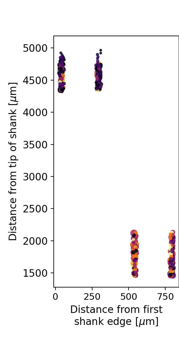
Lets plot the position of each unit overlayed on the shanks. The size of the dots is the spike amplitude, the color is the firing rate.
# get unit metrics, remove positions that could not be computed and use parameter_set_num to select the sorting.
unitmetrics = pd.DataFrame((UnitMetrics & selected_session & 'position != "NULL"' & 'parameter_set_num = 5').fetch())

fig = plt.figure(figsize = [3,6])
fig.add_axes([0.3,0.2,0.7,0.7])

pos = np.vstack(unitmetrics.position.values)
# sort by the inverse of the amplitude so the units are visible
idx = np.argsort(unitmetrics.spike_amplitude.values)[::-1]
plt.scatter(*pos[idx].T,
            unitmetrics.spike_amplitude.values[idx]/10,
            unitmetrics.firing_rate.values[idx], # color by the firing rate
            alpha = 0.8,
            cmap = 'inferno',
            clim = [0,30])
plt.ylabel('Distance from tip of shank [$\\mu$m]');
plt.xlabel('Distance from first\nshank edge [$\\mu$m]');
Working with sorted units
The spike times, amplitudes and positions of each spike are stored in the SpikeSorting.Unit table.
# gets all spikes, positions and amplitudes; the parameter set is the parameters of the sorter.
units = (SpikeSorting.Unit & selected_session & 'parameter_set_num = 5').fetch(as_dict = True)
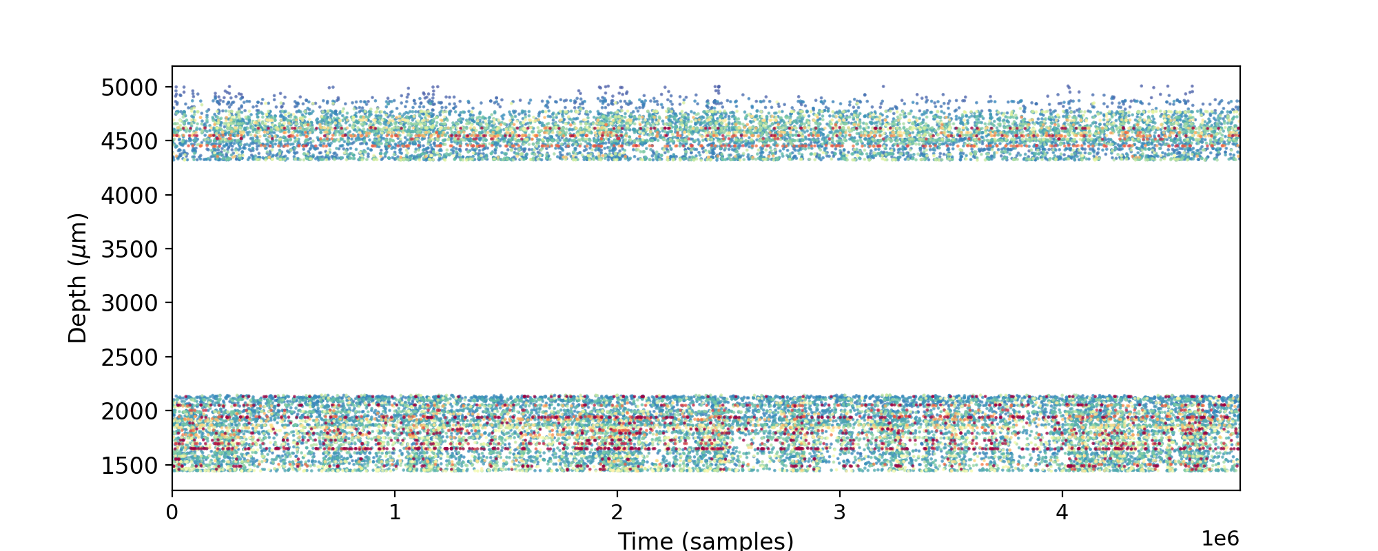
Plot a rastermap
spikes = np.hstack([u['spike_times'] for u in units])
amplitudes = np.hstack([u['spike_amplitudes'] for u in units])
positions = np.vstack([u['spike_positions'] for u in units])
# select a random subset of spikes
idx = np.random.choice(np.arange(len(spikes)),150000)
idx = idx[np.argsort(amplitudes[idx])] # sort by amplitude

fig = plt.figure(figsize=[10,4])
plt.scatter(spikes[idx],positions[idx,1],2,amplitudes[idx],marker = '.',cmap = 'Spectral_r',alpha=0.7,edgecolors=None,clim = [0,20000])
plt.xlim(0,30000*160)
plt.ylabel('Depth ($\\mu$m)')
plt.xlabel('Time (samples)');
To get only the units in a specific shank, one can filter by UnitMetrics
# get the units in a specific shank
units = (SpikeSorting.Unit & (UnitMetrics & 'shank = 2' &
                              selected_session &
                              'parameter_set_num = 5')).fetch(as_dict = True)

spikes = np.hstack([u['spike_times'] for u in units])
amplitudes = np.hstack([u['spike_amplitudes'] for u in units])
positions = np.vstack([u['spike_positions'] for u in units])
# select a random subset of spikes like above
idx = np.random.choice(np.arange(len(spikes)),150000)
idx = idx[np.argsort(amplitudes[idx])] # sort by amplitude

fig = plt.figure(figsize = [3,6])
fig.add_axes([0.3,0.2,0.6,0.7])

plt.scatter(positions[idx,0],positions[idx,1],0.5,amplitudes[idx],
            marker = '.',
            cmap = 'Spectral_r',
            alpha=0.5,
            edgecolors=None,
            clim = [0,20000])
plt.axis('off');
plt.ylabel('Distance from tip of shank [$\\mu$m]');
plt.xlabel('Distance from first\nshank edge [$\\mu$m]');

Accessing syncronized spike-times
Spiketimes are stored as unsigned integer numbers (in samples), to convert to seconds you can:
- divide by the sampling rate (okay if the sampling rate is correct)
- interpolate the times to another stream to get the timing matched between streams that were acquired on different clocks
The method SpikeSorting.Unit.get_spike_times() will get corrected spiketimes in seconds but in order to use the method 2, it requires that the stream sync is specified in the StreamSync object.
This object creates an interpolation function between streams on different clocks; it can be used generically for other streams provided that the same sync signal is recorded across streams.
StreamSync uses the sampled streams in DatasetEvents.Digital. These are populated automatically by the ephys rule, if not they can be added them by calling the EphysRecording.add_nidq_events() method: (EphysRecording & selected_session).add_nidq_events()
To plot synced events:
plt.figure()
(DatasetEvents.Digital() & selected_session).plot_synced();
To add a StreamSync object that can be used to syncronize data acquired with different clocks:
dset_key = (Dataset & (EphysRecording & selected_session)).proj().fetch1()
# add a clock and a stream
StreamSync().insert1(dict(dset_key,
                         stream_name = 'imec0', # the stream we are going to sync
                         event_name = 6, # the common signal recorded on both streams
                         clock_dataset = dset_key['dataset_name'], # dataset where the clock comes from
                         clock_stream = 'nidq',   # stream to be the master clock
                         clock_stream_event = 7)) # the common signal recorded on both streams (channel on master clock)
Note that if one has multiple probes, you should add a stream_name for each probe. To get the spike times already aligned to the recording:
# get the spiketimes already synced because of StreamSync
units = (SpikeSorting.Unit & (UnitMetrics
                              & selected_session
                              & 'parameter_set_num = 5')).get_spike_times()
Working with datafiles and events
Get the events from DatasetEvents.Digital already in sync with the probe because of the StreamSync entry. If the entry is not added, the code will display a warning.
events = pd.DataFrame((DatasetEvents.Digital & selected_session ).fetch_synced()) # get synced dataset events

event_times = events[events['event_name'] == str(1)]['event_timestamps'].iloc[0] # get channel 1
event_values = events[events['event_name'] == str(1)]['event_values'].iloc[0] # because every transition is logged (rise and fall)
event_times = event_times[event_values == 1]
The event times can be combined with a logfile.
Use LIKE to search for files of a specific extension. Note that the % represents any preamble. In the example below, file_path can have any name but must contain orientation followed by .csv.
# Read a log file
log = pd.read_csv((File & (Dataset.DataFiles & selected_session
                   & 'file_path LIKE "%orientation%.csv"')).get()[0])
log['stim_times'] = event_times
stimtimes_sorted = log.sort_values(by='stim')['stim_times'].values
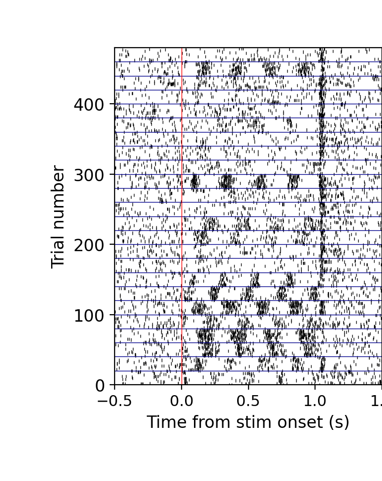
This will plot a raster that can be cicled through using ipywidgets.
# get the spiketimes already synced because of StreamSync
units = (SpikeSorting.Unit & (UnitMetrics  & selected_session & 'parameter_set_num = 5')).get_spike_times()
ts = [u['spike_times'] for u in units]

# get the triggered activity
tpre = 0.5
tpost = 1.5
triggered = []
for sp in ts:
    triggered.append([sp[(sp>(p-tpre)) & (sp<(p+tpost))] - p for p in stimtimes_sorted])

# plot an interactive raster
from spks import plot_raster
fig = plt.figure()
from ipywidgets import interact,IntSlider
@interact(iunit = IntSlider(min=0,max=len(triggered)-1))
def pl(iunit):
  fig.clf()
  plot_raster(triggered[iunit],markersize=5)
  plt.hlines(np.arange(0,len(log),log.trial.max()+1),-tpre,tpost,'darkblue',lw = 0.5)
  plt.vlines(0,0,len(log),'r',lw = 0.5)
  plt.xlabel('Time from stim onset (s)')
  plt.ylabel('Trial number')
Unit counts and criteria for single units
The get_spike_times method can also return the unit metrics so these can be combined easily.
We can also filter the units based on unit metrics. The criteria is defined in the UnitCountCriteria table.
UnitCount.populate() applies criteria to all units and returns the number of single units and multi-units.
UnitCountCriteria().insert1(dict(unit_criteria_id = 1,
                                 # criteria to consider single unit
                                sua_criteria = 'isi_contamination < 0.1 & amplitude_cutoff < 0.1 & spike_duration > 0.1 & spike_amplitude > 50 & presence_ratio > 0.6',
                                # criteria to consider multi unit
                                    mua_criteria = 'spike_duration > 0.01 & n_electrodes_spanned < 20'),
                            skip_duplicates = True)

UnitCount.populate(selected_session) # if you don't select a restriction, it will compute on all datasets.
Select only single units that pass the criteria can be done using the UnitCount.Unit table, remember to specify the unit_criteria_id.
suaunits = (SpikeSorting.Unit & (UnitMetrics*UnitCount.Unit &
                              'passes = 1' &  # use only SUA criteria passing units
                              selected_session &
                              'parameter_set_num = 5')).get_spike_times(include_metrics = True) # return also the metrics
Using the UnitCount table, one can also plot the units versus days on chronic experiments.
# list all subjects with ephys datasets
subjects = (Subject() &( Dataset &  'dataset_type = "ephys"')).proj().fetch(as_dict = True)

subject = subjects[0] # get the first subject

# plot the dates of all recording sessions and the duration
query = (EphysRecording() & subject).proj()

unit_counts = pd.DataFrame((Session*EphysRecording*UnitCount & query).fetch())

import pylab as plt

fig = plt.figure()
for u in np.unique(unit_counts.unit_criteria_id.values):
    subset = unit_counts[unit_counts.unit_criteria_id == u]
    plt.plot(subset.session_datetime.values,subset.sua.values,'-o',alpha = 0.5,label = f'{(UnitCountCriteria & dict(unit_criteria_id = u)).fetch1("sua_criteria")}')
plt.ylim([0,200])
plt.xticks(rotation = 45);
plt.legend(fontsize = 7,loc = 'center left',bbox_to_anchor=(1.05, 1))
Aggregation queries
You can use datajoint's aggr method to compute summary statistics directly on the server, without downloading any data. This is useful for getting quick answers from the database.
For example, to count the total number of single units per recording for a given unit criteria:
EphysRecording.aggr(UnitCount & 'unit_criteria_id = 1', single_unit_count='sum(sua)')
This groups UnitCount entries by each EphysRecording and returns the sum of sua (single unit count) as single_unit_count. You can restrict the result further, for example to a specific subject:
(EphysRecording & subject).aggr(UnitCount & 'unit_criteria_id = 7', single_unit_count='sum(sua)')
Other aggregations work the same way, for example counting the number of sortings per recording:
EphysRecording.aggr(SpikeSorting, n='count(*)')
Imaging
For imaging there are different tables depending on the datatype:
TwoPhotonstores two-photon imaging datasetsWidefieldfor widefield imagingMiniscopefor miniscope imaging (only UCLA miniscope supported at the moment)FixedBrainfor whole brain imaging
For cell segmentation, there are compute tables for both CaimAn and Suite2p that write the results to the CellSegmentation table.
CellSegmentation
Behavior
labdata can also handle behavioral data, aside from videos.
The DecisionMaking table can store data from decision-making tasks; the table is agnostic to the task structure so having the data in this format makes it easy to access different behaviors with the same plotting code.
The populate of the DecisionMaking table are handled by plugins that if appropriate write also to other tables. For example, it is common to have a plugin write to a DatasetVideo (to handle videos), DatasetEvents (to store Digital events or task parameters and synchrize with other datasets) , Weighing (animal weight) or Watering (to store the amount of water consumed) tables.
Plot behavior from all sessions in the DecisionTask
Using the DecisionTask we can pull data and plot the performance on easy trials for all sessions that are available in the database.
from labdata.schema import *  # import tables
import pylab as plt           # for plotting

# List the mice with decision task
mice = (Subject & DecisionTask()).fetch('KEY')
print(f'There are {len(mice)} subjects that ran at least one session.')
# list the number of sessions per animal with an AGGREGATE call
pd.DataFrame(Subject.aggr(DecisionTask,number_of_sessions = 'count(subject_name)'))
The DecisionTask table contains number of trials performed during the session and other information like the amount of water consumed. The DecisionTask.TrialSet table contains subsets of trials for which the experimental conditions where similar; and stores performance, intensity of the stimulus, response of the subject, etc.
The following code plots the performance on each session with trial_set_description = "visual" but only for sessions that had more than 100 performed trials. Lets use the performance_easy that contains the performance on easy trials only.
colors = plt.cm.tab20(np.linspace(0,1,len(mice)))
plt.figure(figsize = (10,2))
for i,m in enumerate(mice):
  # we need performance_easy and session_datetime. we do this only for visual trial sets
  # plot only for >100 sessions with over 100 performed trials
  dates,perf = ((DecisionTask*DecisionTask.TrialSet*Session &  m
                 & 'trialset_description = "visual"'
                 & 'n_total_performed > 100')).fetch('session_datetime', 'performance_easy')
  if len(dates): # exclude mice that had no sessions for the query
    plt.plot(dates,perf,'o-',markersize = 3,color = colors[i],label = m['subject_name'],alpha = 0.8)
    # write the subject name next to the data
    plt.text(np.random.choice(dates[:20],1),
             np.random.uniform(0.8,1.1,1),m['subject_name'],
             fontsize = 6,
             fontweight = 'bold', color = colors[i])
plt.ylim([0,1])
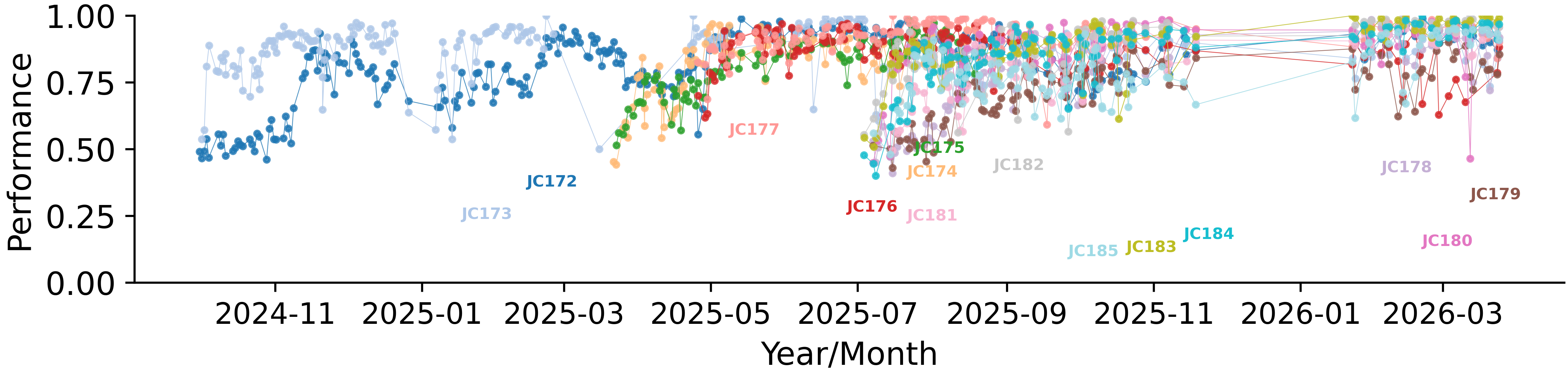
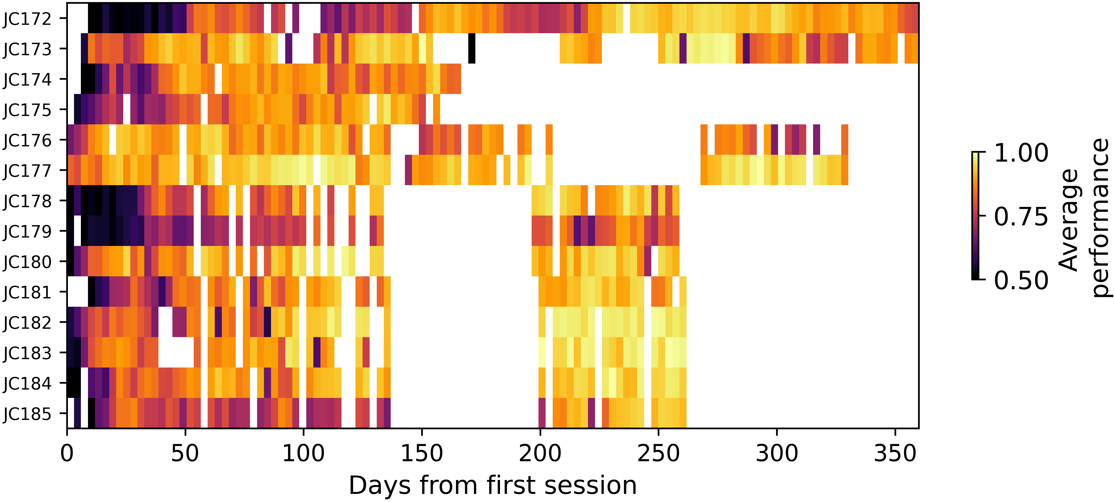
This plot is not very informative because the curves overlay and the axis is not normalized for all subjects. Lets instead plot an histogram of average performance over days since the first session.
binsize = 3                     # in days
ed = np.arange(0,365,binsize)   # the bin edges
performance = np.stack([np.zeros(ed.shape[0]-1)]*len(mice))
performance[:] = np.nan
for i,m in enumerate(mice):
    dates,perf = ((DecisionTask*DecisionTask.TrialSet*Session &  m
                 & 'trialset_description = "visual"'
                 & 'n_total_performed > 100')).fetch('session_datetime', 'performance_easy')
    # get the start date of the first session logged in DecisionTask
    start_date = (Subject & m).aggr(DecisionTask*Session,first_session = 'min(session_datetime)').fetch1('first_session')
    if len(dates): # exclude mice that had no sessions for that condition
        days = (dates-start_date).astype('timedelta64[D]').astype(int)      # days from start
        from scipy.stats import binned_statistic
        vals = binned_statistic(days,perf,bins = ed, statistic='mean')[0]   # compute the average performance in each bin
        performance[i] = vals
# plot the data
fig = plt.figure(figsize = [10,4])
fig.add_axes([0.1,0.2,0.7,0.7])
plt.imshow(performance,cmap = 'inferno',extent = [0,ed[-2],len(performance),0],clim = [0.5,1],aspect = 'auto')
# set the ticks to the name of the subjects
plt.yticks(np.arange(performance.shape[0])+0.5,[m['subject_name'] for m in mice],fontsize = 8);
plt.colorbar(shrink = 0.3,label='Average performance')
plt.xlabel('Days from first session');